109. A Linear Model of Unemployment#
GPU
This lecture was built using a machine with access to a GPU — although it will also run without one.
Google Colab has a free tier with GPUs that you can access as follows:
Click on the “play” icon top right
Select Colab
Set the runtime environment to include a GPU
In addition to what’s in Anaconda, this lecture needs the following libraries.
We first install numpyro and jax:
!pip install numpyro jax
We also install pandas_datareader, which we use to download data from FRED:
!pip install pandas_datareader
109.1. Overview#
This lecture fits some simple time series models to the US unemployment rate.
Our aim is partly to practice Bayesian estimation on real data, and partly to find out what these simple models cannot do — which will motivate the richer model in the sequel Bayesian Estimation of Nonlinear Unemployment Dynamics.
We met Bayesian estimation of a first-order autoregression (AR(1)) in Posterior Distributions for AR(1) Parameters, but there the data were simulated and the focus was on the initial condition.
Here the data are real, and we try to describe them with an AR(1) model.
We will see how well that description works and where it breaks down.
We’ll also ask whether or not unemployment is a random walk, which is a special case of the AR(1) model.
That last question is not just a technical curiosity — it was the subject of a lively macroeconomics debate in the 1980s and 1990s.
The natural rate hypothesis [Friedman, 1968] holds that unemployment fluctuates around a stable equilibrium rate, so shocks fade away and the series is stationary.
The hysteresis hypothesis [Blanchard and Summers, 1986] holds the opposite — that shocks to unemployment can be more or less permanent, so the series behaves like a random walk with no fixed level to return to.
(Interestingly, the paper that launched the unit-root literature [Nelson and Plosser, 1982] found that, of fourteen US macroeconomic series, the unemployment rate was the one it could confidently call stationary — even as the hysteresis literature was arguing the reverse for Europe.)
We will see that this debate is genuinely hard to settle.
As in Posterior Distributions for AR(1) Parameters and Non-Conjugate Priors we sample posteriors with the NUTS sampler in NumPyro; see Non-Conjugate Priors for a brief account of how NUTS works.
Our plan is:
look at the data,
consider the simplest model — a random walk — and see what works and what doesn’t,
add mean reversion to get a linear model and estimate it,
ask whether the data really want a random walk after all, and
lay out what is unsatisfying about the linear model.
Let’s start with some imports.
import numpy as np
import matplotlib.pyplot as plt
import datetime as dt
from pandas_datareader import data as web

import jax.numpy as jnp
from jax import random
import numpyro
import numpyro.distributions as dist
from numpyro.infer import MCMC, NUTS
109.2. The data#
We use the US civilian unemployment rate, series UNRATE from FRED, monthly and seasonally adjusted.
We download the whole post-war record.
start, end = dt.datetime(1948, 1, 1), dt.datetime(2024, 12, 31)
unrate = web.DataReader("UNRATE", "fred", start, end)["UNRATE"]
The COVID-19 spike of 2020 is an extreme outlier driven by events the model knows nothing about, so we drop it.
We keep two versions of the series: the monthly data, and an annual series formed from end-of-year values.
pre_covid = unrate[unrate.index < "2020-01-01"]
u_monthly = pre_covid.to_numpy()
u_annual = pre_covid.resample("YE").last().to_numpy()
print(f"monthly: {len(u_monthly)} obs, annual: {len(u_annual)} obs")
monthly: 864 obs, annual: 72 obs
Here are the two series.
fig, (axL, axR) = plt.subplots(1, 2, figsize=(11, 4))
axL.plot(pre_covid.index, u_monthly, lw=2)
axL.set_title('monthly')
axL.set_xlabel('year')
axL.set_ylabel('unemployment rate (%)')
axR.plot(pre_covid.resample("YE").last().index, u_annual, lw=2)
axR.set_title('annual')
axR.set_xlabel('year')
plt.show()
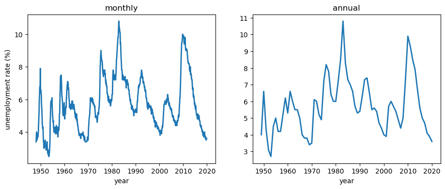
The rate rises sharply in recessions and drifts down in recoveries, but it always stays inside a band — roughly 3% to 11% over the whole post-war period.
Any sensible model has to respect that band.
109.3. A random walk?#
The simplest dynamic model just says that next period equals this period plus a shock,
This is a random walk.
It is worth taking seriously because, as we will see, the data come surprisingly close to it.
But as a description of unemployment it has a fatal flaw.
Under a random walk, \(u_t = u_0 + \sum_{s=1}^t \varepsilon_s\), so the variance of \(u_t\) grows without bound: \(\operatorname{Var}(u_t) = t\sigma^2\).
The distribution spreads out forever, and eventually probability mass drains out of every bounded interval.
We can see the spreading by simulating many random-walk paths and watching them fan out.
rng = np.random.default_rng(0)
T = len(u_monthly)
σ_rw = np.diff(u_monthly).std()
paths = u_monthly[0] + np.cumsum(rng.normal(0, σ_rw, size=(400, T)), axis=1)

fig, ax = plt.subplots()
ax.plot(paths[:60].T, color='C0', lw=0.5, alpha=0.3)
lo, hi = np.percentile(paths, [5, 95], axis=0)
ax.fill_between(np.arange(T), lo, hi, color='C0', alpha=0.2,
                label='90% band')
ax.plot(u_monthly, 'k', lw=2, label='observed')
ax.set_xlabel('months since 1948')
ax.set_ylabel('unemployment rate (%)')
ax.legend()
plt.show()
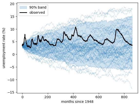
The simulated band widens like \(\sqrt{t}\) and soon covers negative rates and rates above 15%, while the actual series stays in its narrow band.
A random walk has no anchor, but unemployment clearly has one.
109.4. Adding mean reversion#
To give the series an anchor we let it be pulled back toward a normal level \(\bar u\),
with \(0 \le \phi < 1\).
This is a linear AR(1) model for unemployment, written so that \(\bar u\) is the level it reverts to and \(\phi\) measures persistence.
The random walk is the special case \(\phi = 1\), where the pull vanishes.
The smaller \(\phi\), the faster the series returns to \(\bar u\) after a shock.
We give \(\phi\) a uniform prior on \([0, 1)\), so we let the data decide how close to a random walk we are.
def linear_model(u):
    ubar = numpyro.sample("ubar",  dist.Normal(5.5, 2.0))
    φ    = numpyro.sample("phi",   dist.Uniform(0.0, 1.0))
    σ    = numpyro.sample("sigma", dist.HalfNormal(1.0))
    μ = ubar + φ * (u[:-1] - ubar)
    numpyro.sample("u_obs", dist.Normal(μ, σ), obs=u[1:])
We sample the posterior with NUTS, running four chains so we can check convergence.
We use chain_method="vectorized", which evaluates all chains together on a single device, so the same code runs unchanged on a CPU or a GPU.
def run_nuts(model, data, seed=0, num_warmup=1000, num_samples=2000, num_chains=4):
    "Sample a NumPyro model with the NUTS sampler."
    mcmc = MCMC(NUTS(model),
                num_warmup=num_warmup, num_samples=num_samples,
                num_chains=num_chains, chain_method="vectorized",
                progress_bar=False)
    mcmc.run(random.PRNGKey(seed), jnp.asarray(data))
    return mcmc
We fit the model to the monthly data first.
mcmc_monthly = run_nuts(linear_model, u_monthly)
The chains mix well, and here is the posterior summary.
mcmc_monthly.print_summary()
                mean       std    median      5.0%     95.0%     n_eff     r_hat
       phi      0.99      0.00      0.99      0.99      1.00   3607.29      1.00
     sigma      0.21      0.01      0.21      0.20      0.22   4086.14      1.00
      ubar      5.66      1.17      5.69      3.72      7.51   3250.21      1.00

Number of divergences: 0
We then fit it to the annual data.
mcmc_annual = run_nuts(linear_model, u_annual)
Here is the corresponding summary.
mcmc_annual.print_summary()
                mean       std    median      5.0%     95.0%     n_eff     r_hat
       phi      0.81      0.08      0.81      0.68      0.94   3759.20      1.00
     sigma      1.05      0.09      1.04      0.91      1.20   4543.65      1.00
      ubar      5.69      0.80      5.70      4.42      6.91   2839.06      1.00

Number of divergences: 0
109.5. Is it a random walk after all?#
The persistence parameter \(\phi\) tells the story, so we compare its posterior across the two frequencies.
φ_m = np.asarray(mcmc_monthly.get_samples()["phi"])
φ_a = np.asarray(mcmc_annual.get_samples()["phi"])

fig, ax = plt.subplots()
ax.hist(φ_m, bins=50, density=True, alpha=0.6, label='monthly')
ax.hist(φ_a, bins=50, density=True, alpha=0.6, label='annual')
ax.set_xlabel('$\\phi$')
ax.legend()
plt.show()
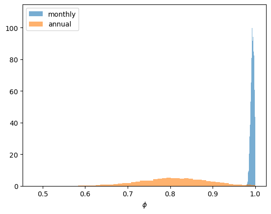
At the monthly frequency the posterior for \(\phi\) crowds right up against one — the random-walk boundary.
In other words, month to month, US unemployment is almost a random walk: the pull back toward \(\bar u\) is barely detectable.
Two summaries make the point.
The model has a stationary distribution \(N\!\big(\bar u,\ \sigma^2/(1-\phi^2)\big)\), and a shock has a half-life of \(\ln 0.5 / \ln \phi\) periods.
def describe(mcmc, label):
    p = mcmc.get_samples()
    φ, σ = np.asarray(p["phi"]), np.asarray(p["sigma"])
    half_life = np.log(0.5) / np.log(φ)
    stat_sd = σ / np.sqrt(1 - φ**2)
    print(f"{label}:")
    print(f"  φ          median {np.median(φ):.3f}  90% [{np.percentile(φ,5):.3f}, {np.percentile(φ,95):.3f}]")
    print(f"  half-life  median {np.median(half_life):.0f} periods")
    print(f"  stationary sd of u: median {np.median(stat_sd):.2f} pp")

describe(mcmc_monthly, "monthly")
describe(mcmc_annual, "annual")
monthly:
  φ          median 0.994  90% [0.986, 0.999]
  half-life  median 107 periods
  stationary sd of u: median 1.83 pp
annual:
  φ          median 0.810  90% [0.676, 0.938]
  half-life  median 3 periods
  stationary sd of u: median 1.78 pp
At the monthly frequency the half-life of a shock runs to several years.
Over a sample of a few hundred months the series barely has time to revert, so it behaves, for practical purposes, like the random walk we just rejected.
At the annual frequency the picture is better: \(\phi\) sits well below one and shocks die out within a few years.
The lesson is that whether unemployment “looks like a random walk” depends on how often you look.
Note
This is exactly the question behind the natural rate versus hysteresis debate of the 1980s and 1990s [Blanchard and Summers, 1986, Friedman, 1968].
When \(\phi\) is this close to one, the debate is hard to settle: in samples of the length we have, a true random walk and a slowly-reverting series look almost the same, so the statistical tests have little power to tell them apart [Røed, 1997].
One way forward, which we take in Bayesian Estimation of Nonlinear Unemployment Dynamics, is to let the reversion be nonlinear — a series can look like a random walk to a linear test while reverting briskly once it strays far enough from its normal level [Kapetanios et al., 2003].
109.6. Random walk, yet recurrent#
The linear model is a clear improvement on the random walk — it has an anchor and a stationary distribution.
But at the frequencies we care about it is barely an improvement: \(\phi\) sits so close to one that the anchor does almost no work, and over realistic horizons the series still behaves much like the random walk we rejected.
This leaves us with a genuine tension.
Read through a linear lens, the data look like a random walk.
But a random walk wanders off without limit, whereas unemployment has stayed in a narrow band for seventy-five years.
The linear model can reconcile these two facts, but only by setting \(\phi\) a hair below one — a knife-edge value the data cannot distinguish from one, and one that imposes the same gentle reversion at all times.
A more robust reconciliation is to let the reversion be nonlinear.
The series can then drift like a random walk in normal times, while a restoring force that strengthens far from the natural rate keeps it from ever wandering away.
Recurrence then comes from the shape of the dynamics in the tails, not from a precise value of \(\phi\) — and the series can be genuinely random-walk-like exactly where we usually observe it.
To set up what comes next, it helps to look at the restoring force directly, by plotting each one-step change against the gap that preceded it, with the fitted linear pull overlaid.
ubar_hat = np.median(np.asarray(mcmc_annual.get_samples()["ubar"]))
φ_hat = np.median(φ_a)
gap = u_annual[:-1] - ubar_hat
Δu = np.diff(u_annual)

fig, ax = plt.subplots()
ax.scatter(gap, Δu, alpha=0.6, label='annual data')
gg = np.linspace(gap.min(), gap.max(), 100)
ax.plot(gg, (φ_hat - 1) * gg, 'C1', lw=2, label='linear pull')
ax.axhline(0, color='k', lw=.5)
ax.axvline(0, color='k', lw=.5)
ax.set_xlabel('gap $u_t - \\bar u$')
ax.set_ylabel('change $\\Delta u$')
ax.legend()
plt.show()
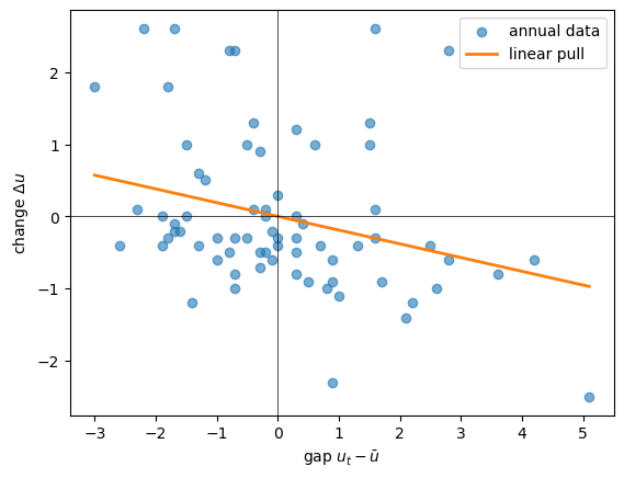
The straight line is a reasonable summary of the average reversion in the data.
Whether a force that is gentle near the center but firmer far from it fits better — and whether the data can even tell — is the question we take up in Bayesian Estimation of Nonlinear Unemployment Dynamics.
109.7. Exercises#
The lecture Forecasting an AR(1) Process forecasts an AR(1) process by simulating future paths, and draws a careful distinction between a predictive distribution that conditions on fixed parameter values and one that integrates over their posterior uncertainty.
The following exercises apply that methodology to our fitted unemployment model.
Exercise 109.1
Using the fitted annual model, forecast unemployment over the next \(H = 15\) years, starting from the last observed value, in two ways:
plug-in: hold the parameters at their posterior medians and simulate many future paths;
extended: for each future path, draw a fresh \((\bar u, \phi, \sigma)\) from the posterior.
Plot the 90% predictive band for each on the same axes and compare.
Which band is wider, and why?
Solution
We use the annual posterior draws and simulate forward from the last observation.
We work with the annual model because its persistence \(\phi\) is far less certain than at the monthly frequency, so parameter uncertainty has more to say.
post = mcmc_annual.get_samples()
ubar_s = np.asarray(post["ubar"])
φ_s = np.asarray(post["phi"])
σ_s = np.asarray(post["sigma"])

def sim_future(u_last, ubar, φ, σ, H, rng):
    "Simulate H steps of the linear model forward from u_last."
    u = np.empty(H)
    prev = u_last
    for h in range(H):
        prev = ubar + φ * (prev - ubar) + rng.normal(0, σ)
        u[h] = prev
    return u

H, N = 15, 2000
u_last = u_annual[-1]
rng = np.random.default_rng(0)

# plug-in: parameters fixed at posterior medians
ub0, φ0, σ0 = np.median(ubar_s), np.median(φ_s), np.median(σ_s)
plug = np.array([sim_future(u_last, ub0, φ0, σ0, H, rng) for _ in range(N)])

# extended: a fresh posterior draw for each path
idx = rng.integers(0, len(φ_s), N)
ext = np.array([sim_future(u_last, ubar_s[i], φ_s[i], σ_s[i], H, rng)
                for i in idx])

fig, ax = plt.subplots()
horizon = np.arange(1, H + 1)
for data, c, lab in [(plug, 'C0', 'plug-in'), (ext, 'C1', 'extended')]:
    lo, hi = np.percentile(data, [5, 95], axis=0)
    ax.fill_between(horizon, lo, hi, alpha=0.3, color=c, label=lab)
ax.axhline(u_last, color='k', lw=0.5)
ax.set_xlabel('years ahead')
ax.set_ylabel('unemployment rate (%)')
ax.legend()
plt.show()
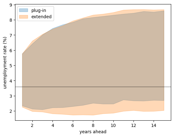
Both forecasts drift up from the low starting value toward the reversion level \(\bar u\), with bands that widen as we look further ahead.
The extended band is clearly wider, because it adds uncertainty about the parameters on top of the uncertainty from future shocks — and here the persistence \(\phi\) and the level \(\bar u\) are both genuinely uncertain.
Exercise 109.2
Following Wecker (see Forecasting an AR(1) Process), we can also form a predictive distribution for a path statistic — a nonlinear function of the whole future path.
Take the maximum unemployment rate over the next \(H = 8\) years as the statistic: a simple measure of how bad the next several years might get.
Using the extended simulation (a posterior draw per path), compute this maximum for each path and plot its predictive distribution.
What is the posterior predictive probability that unemployment reaches at least \(7\%\) — recession territory — at some point over the next eight years?
Solution
We reuse sim_future and the posterior draws from the previous exercise.
H2, M = 8, 5000
idx = rng.integers(0, len(φ_s), M)
peak = np.array([sim_future(u_last, ubar_s[i], φ_s[i], σ_s[i], H2, rng).max()
                 for i in idx])

fig, ax = plt.subplots()
ax.hist(peak, bins=50, density=True, alpha=0.6)
ax.axvline(u_last, color='C3', lw=2, label='current rate')
ax.set_xlabel('maximum unemployment over next 8 years (%)')
ax.legend()
plt.show()

prob = (peak > 7.0).mean()
print(f"P(unemployment reaches 7% within 8 years) = {prob:.2f}")
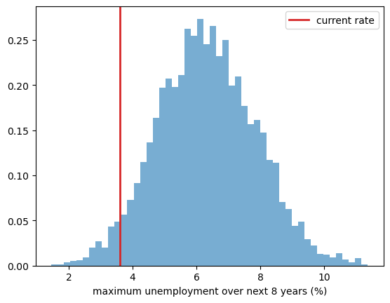
P(unemployment reaches 7% within 8 years) = 0.32
The predictive distribution summarizes the plausible “worst case” over the next several years, integrating over both shocks and parameter uncertainty.
Starting from a cyclical low, the model sees a substantial chance of a return to recession-level unemployment within the horizon.